Code Example

Demo code for the paper "Whole-brain B₁-mapping using three dimensional DREAM" by Philipp Ehses, Daniel Brenner, Rüdiger Stirnberg, Eberhard Pracht, and Tony Stöcker.

Dependencies:

python/ipython 2.x or 3.x
argparse
numpy
matplotlib
nibabel

# import of external libraries & general configuration

# python 2 & 3 compatible:
from __future__ import division, print_function

import os
import numpy as np
import matplotlib as mpl
import matplotlib.pyplot as plt
import nibabel as nib
# os.chdir("/home/jovyan/content/03/")

mpl.rcParams['font.size'] = 12
mpl.rcParams['figure.titlesize'] = 16
mpl.rcParams['axes.titlesize'] = 14
mpl.rcParams['xtick.labelsize'] = 12
mpl.rcParams['ytick.labelsize'] = 12

Load data and show raw images

The dimensions in the nifti file are in the following order:

first phase encoding
read/frequency encoding
second phase encoding
repetitions (STE, FID)

This order is very important for the blurring compensation later. To simplify the rest of reconstruction process, we make sure that the two phase-encoding directions are in the first two dimensions of the numpy arrays dream_r1 and dream_r4.

dream_r1 = nib.load('3DREAM_R1.nii.gz').get_fdata()
dream_r4 = nib.load('3DREAM_R4.nii.gz').get_fdata()

# make sure that phase-encoding directions are in first two dimensions:
dream_r1 = np.moveaxis(dream_r1, 2, 1)
dream_r4 = np.moveaxis(dream_r4, 2, 1)

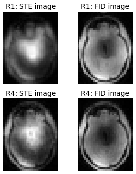
zpos = 24

fig = plt.figure(figsize=(5,6));

plt.subplot(221);
plt.title('R1: STE image');
plt.imshow(dream_r1[:,:,zpos,0], cmap='gray');
plt.axis('off');

plt.subplot(222);
plt.title('R1: FID image');
plt.imshow(dream_r1[:,:,zpos,1], cmap='gray');
plt.axis('off');

plt.subplot(223);
plt.title('R4: STE image');
plt.imshow(dream_r4[:,:,zpos,0], cmap='gray');
plt.axis('off');

plt.subplot(224);
plt.title('R4: FID image');
plt.imshow(dream_r4[:,:,zpos,1], cmap='gray');
plt.axis('off');

You should be able to appreciate how the higher acceleration factor helps to reduce blurring (especially in the STE image).

Conventional DREAM flip angle map

The preparation flip angle alpha can be obtained from the two contrasts according to Nehrke et al. 2012:

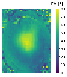
def calc_fa(ste, fid):
    famap = np.rad2deg(np.arctan(np.sqrt(2. * ste/fid)))
    return famap

fa_r1 = calc_fa(dream_r1[:,:,:,0], dream_r1[:,:,:,1])
fa_r4 = calc_fa(dream_r4[:,:,:,0], dream_r4[:,:,:,1])


fig, axes = plt.subplots(nrows=1, ncols=2);
fig.suptitle("Flip angle maps");

axes[0].set_title('R = 1');
axes[0].imshow(fa_r1[:,:,zpos], cmap='viridis', vmin=0, vmax=80);
axes[0].axis('off');

axes[1].set_title('R = 4');
im = axes[1].imshow(fa_r4[:,:,zpos], cmap='viridis', vmin=0, vmax=80);
axes[1].axis('off');

fig.subplots_adjust(right=0.85);
cbar_ax = fig.add_axes([0.9, 0.25, 0.035, 0.5]);
cbar_ax.set_title('FA [°]', pad=12);
fig.colorbar(im, cax=cbar_ax);

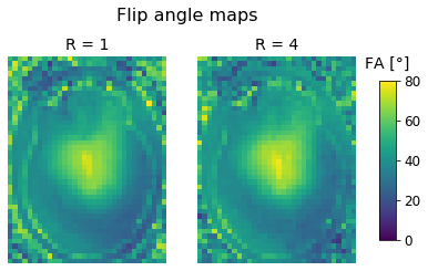
A bright ring around the brain is clearly visible in both maps, but it appears more pronounced in the unaccelerated data.

This ring is a result of the different blurring levels that are present in the STE and FID images (dividing differently blurred images by one another is not such a great idea).

Blurring Compensation

In order to compensate for the stronger blurring in the STE image, we first need some information about sequence parameters and the phase-encoding order.

from DreamMap import approx_sampling, global_filter, local_filter, image_to_kspace, kspace_to_image

# we need some information about the sequence:
tr = 3.06e-3
alpha = 60          # preparation FA
beta = 6            # readout FA
dummies = 1         # number of dummy scans before readout echo train starts
etl_r1 = 1049       # echo train length for R = 1
etl_r4 = 266        # echo train length for R = 4
etd_r1 = etl_r1*tr  # echo train duration for R = 1
etd_r4 = etl_r4*tr  # echo train duration for R = 4


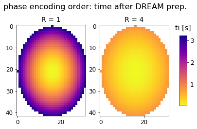
# we also need to estimate the "inversion time" ti (analogue to IR experiments)
# i.e. the time after DREAM preparation after which each k-space line is acquired
# to do this, there's a helper function that approximates the spiral-out PE order:
ti_r1 = approx_sampling(dream_r1.shape[:2], etl_r1, tr, dummies)
ti_r4 = approx_sampling(dream_r4.shape[:2], etl_r4, tr, dummies)


fig, axes = plt.subplots(nrows=1, ncols=2);
fig.suptitle("phase encoding order: time after DREAM prep.");

axes[0].set_title('R = 1');
axes[0].imshow(ti_r1, cmap='plasma_r', vmin=np.nanmin(ti_r1), vmax=np.nanmax(ti_r1));
# axes[0].axis('off')

axes[1].set_title('R = 4');
im = axes[1].imshow(ti_r4, cmap='plasma_r', vmin=np.nanmin(ti_r1), vmax=np.nanmax(ti_r1));
# axes[1].axis('off')

fig.subplots_adjust(right=0.85);
cbar_ax = fig.add_axes([0.9, 0.25, 0.035, 0.5]);
cbar_ax.set_title('ti [s]', pad=12);
fig.colorbar(im, cax=cbar_ax);

Global blurring compensation technique

First, let's calculate a global filter window for the FID signal that can be used to approximate blurring that is present in the STEAM image. For this, we need the average tissue T1, the phase encoding order (or time after STEAM preparation, "ti") as well as other sequence parameters (TR, and flip angles $\alpha$ and $\beta$):

def DREAM_filter_window(alpha, beta, tr, t1, ti):

    # from degrees to radians:
    alpha = np.deg2rad(alpha)
    beta = np.deg2rad(beta)
    
    # initial STEAM signal after preparation:
    S0_STE = np.sin(beta) * np.sin(alpha)**2
    
    # initial FID signal after preparation:
    S0_FID = np.sin(beta) * np.cos(alpha)**2
    
    # FID steady-state signal:
    Sstst = np.sin(beta) * (1 - np.exp(-tr / t1)) / (1 - np.cos(beta) * np.exp(-tr / t1))
    
    # effective relaxation rate that describes signal evolution after preparation:
    r1s = 1/t1 - np.log(np.cos(beta))/tr
    
    ## signal evolution for STEAM and FID:
    # S_STE(ti) = S0_STE * exp(-r1s*ti)                      # exponential decay
    # S_FID(ti) = Sstst + (S0_FID - Sstst) * exp(-r1s * ti)  # evolution from S0_FID towards Sstst
    
    # the appropriate window function for the FID image that results in similar blurring as in STEAM is given by
    # the ratio of the two evolution curves normalized to their initial value: (S_STE/S0_STE)/(S_FID/S0_FID).
    
    # After simplification, this results in:    
    filter_window = S0_FID/(S0_FID + Sstst*(np.exp(r1s*ti)-1.))
    
    # if ti==0 assume that this data was not acquired and set the window to zero
    filter_window[np.isnan(ti)] = 0
    
    return filter_window


ste = dream_r1[:,:,:,0]
fid = dream_r1[:,:,:,1]

\ With this helper function, we can now calculate a global window function for a given experiment.

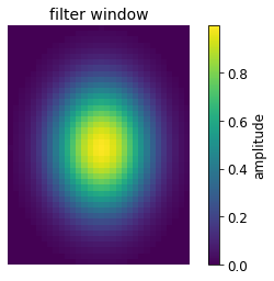
Let's start with the unaccelerated data. Since, this filter is applied to the whole 3D volume, we need global flip angle and $T_1$ estimates. For $T_1$, let's choose 2 s which is close to the gray matter $T_1$ at 7T (and in between white matter and CSF). For the flip angle, let's use the average STEAM and FID signal in order to calculate a flip angle $\alpha$ estimate from Equation 1.

# choose unaccelerated data:
ste = dream_r1[:,:,:,0]
fid = dream_r1[:,:,:,1]

# t1 and flip angle estimates:
t1  = 2.   # [s] - approximately gray matter T1 @ 7T
mean_alpha = calc_fa(ste.mean(), fid.mean())
mean_beta = mean_alpha / alpha * beta

# calculate filter window
filter_window = DREAM_filter_window(mean_alpha, mean_beta, tr, t1, ti_r1)

# plot filter window
plt.title('filter window')
plt.imshow(filter_window)
plt.axis('off')
plt.colorbar(label='amplitude')

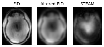
<matplotlib.colorbar.Colorbar at 0x7f23811787d0>

\ \ Now let's apply this filter window and compare the resulting blurred FID image with the STEAM and original FID image:

# ifft in lin & par spatial dims
sig = image_to_kspace(fid, [0, 1])
       
# multiply with filter
sig *= filter_window[:,:,np.newaxis]

fid_filt = abs(kspace_to_image(sig, [0, 1]))

fig, axes = plt.subplots(nrows=1, ncols=3);

axes[0].set_title('FID');
axes[0].imshow(abs(fid[:,:,zpos]), cmap='gray', vmax=0.25);
axes[0].axis('off');

axes[1].set_title('filtered FID');
axes[1].imshow(fid_filt[:,:,zpos], cmap='gray', vmax=0.25);
axes[1].axis('off');

axes[2].set_title('STEAM');
axes[2].imshow(ste[:,:,zpos], cmap='gray', vmax=0.2);
axes[2].axis('off');

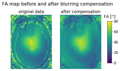
\ Now that we have an FID image with a level of blurring that resembles the STEAM, we can calculate the flip angle map and compare it to the original map:

fig, axes = plt.subplots(nrows=1, ncols=2);
fig.suptitle("FA map before and after blurring compensation");

axes[0].set_title('original data');
axes[0].imshow(fa_r1[:,:,zpos], cmap='viridis', vmin=0, vmax=80);
axes[0].axis('off');

global_r1 = abs(calc_fa(ste, fid_filt))
axes[1].set_title('after compensation');
im = axes[1].imshow(global_r1[:,:,zpos], cmap='viridis', vmin=0, vmax=80);
axes[1].axis('off');

fig.subplots_adjust(right=0.85);
cbar_ax = fig.add_axes([0.9, 0.25, 0.035, 0.5]);
cbar_ax.set_title('FA [°]', pad=12);
fig.colorbar(im, cax=cbar_ax);

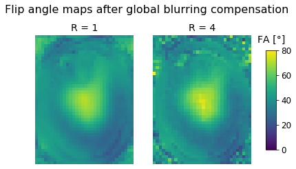
\ Let's repeat this for the unaccelerated and accelerated data and compare the results:

ste, fid = global_filter(dream_r1[:,:,:,0], dream_r1[:,:,:,1], ti_r1, alpha, beta, tr, t1)
global_r1 = calc_fa(ste, fid)
ste, fid = global_filter(dream_r4[:,:,:,0], dream_r4[:,:,:,1], ti_r4, alpha, beta, tr, t1)
global_r4 = calc_fa(ste, fid)

fig, axes = plt.subplots(nrows=1, ncols=2);
fig.suptitle("Flip angle maps after global blurring compensation");

axes[0].set_title('R = 1');
axes[0].imshow(global_r1[:,:,zpos], cmap='viridis', vmin=0, vmax=80);
axes[0].axis('off');

axes[1].set_title('R = 4');
im = axes[1].imshow(global_r4[:,:,zpos], cmap='viridis', vmin=0, vmax=80);
axes[1].axis('off');

fig.subplots_adjust(right=0.85);
cbar_ax = fig.add_axes([0.9, 0.25, 0.035, 0.5]);
cbar_ax.set_title('FA [°]', pad=12);
fig.colorbar(im, cax=cbar_ax);

The ring around the brain seems to be gone now in both datasets.

Local iterative blurring compensation technique

We use the global compensated maps as an initial guess (fmap=global_rX).

ste, fid = local_filter(dream_r1[:,:,:,0], dream_r1[:,:,:,1], ti_r1, alpha, beta, tr, t1, fmap=global_r1)
local_r1 = calc_fa(ste, fid)
ste, fid = local_filter(dream_r4[:,:,:,0], dream_r4[:,:,:,1], ti_r4, alpha, beta, tr, t1, fmap=global_r4)
local_r4 = calc_fa(ste, fid)

fig, axes = plt.subplots(nrows=1, ncols=2);
fig.suptitle("Flip angle maps after local iterative blurring compensation");

axes[0].set_title('R = 1');
axes[0].imshow(local_r1[:,:,zpos], cmap='viridis', vmin=0, vmax=80);
axes[0].axis('off');

axes[1].set_title('R = 4');
im = axes[1].imshow(local_r4[:,:,zpos], cmap='viridis', vmin=0, vmax=80);
axes[1].axis('off');

fig.subplots_adjust(right=0.85);
cbar_ax = fig.add_axes([0.9, 0.25, 0.035, 0.5]);
cbar_ax.set_title('FA [°]', pad=12);
fig.colorbar(im, cax=cbar_ax);

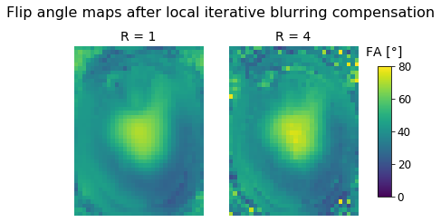
On first glance, this looks very similar to the global compensation technique. However, as our analysis in the paper shows, there is still a slight improvement that only costs us a small amount of computation time. Still, the global compensation technique is a viable option in case a simple and very fast compensation technique is required.

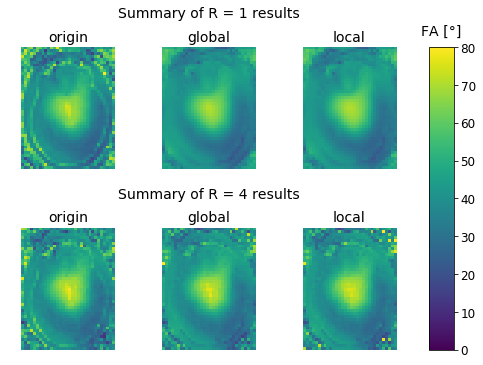
Summary of the Results

plt.figure(figsize=(8,6));
gs = mpl.gridspec.GridSpec(nrows = 5, ncols = 4, width_ratios=[1, 1, 1, 0.2], height_ratios=[0.1, 1., 0.1, 0.1, 1.]);

ax_t1 =  plt.subplot(gs[0,:-1]);
ax_t1.set_title("Summary of R = 1 results");
ax_t1.axis('off');

ax1 = plt.subplot(gs[1,0]);
ax1.set_title('origin');
ax1.imshow(fa_r1[:,:,zpos], cmap='viridis', vmin=0, vmax=80);
ax1.axis('off');

ax2 = plt.subplot(gs[1,1]);
ax2.set_title('global');
ax2.imshow(global_r1[:,:,zpos], cmap='viridis', vmin=0, vmax=80);
ax2.axis('off');

ax3 = plt.subplot(gs[1,2]);
ax3.set_title('local');
ax3.imshow(local_r1[:,:,zpos], cmap='viridis', vmin=0, vmax=80);
ax3.axis('off');

ax_t2 =  plt.subplot(gs[3,:-1]);
ax_t2.set_title("Summary of R = 4 results");
ax_t2.axis('off');

ax4 = plt.subplot(gs[4,0]);
ax4.set_title('origin');
ax4.imshow(fa_r4[:,:,zpos], cmap='viridis', vmin=0, vmax=80);
ax4.axis('off');

ax5 = plt.subplot(gs[4,1]);
ax5.set_title('global');
ax5.imshow(global_r4[:,:,zpos], cmap='viridis', vmin=0, vmax=80);
ax5.axis('off');

ax6 = plt.subplot(gs[4,2]);
ax6.set_title('local');
im = ax6.imshow(local_r4[:,:,zpos], cmap='viridis', vmin=0, vmax=80);
ax6.axis('off');


cbar_ax = plt.subplot(gs[1:,3]);
cbar_ax.set_title('FA [°]', pad=12);
fig.colorbar(im, cax=cbar_ax);

Command line interface

DreamMap.py also has a command line interface that allows the direct calculation of flip angle maps from nifti files that include the two contrasts (STE & FID). The following system call will give us the uncorrected flip angle map, the global compensated, as well as the local iterative compensated map.

Here are the availaible arguments that can be passed to the script:

Running the script

DreamMap.py requires the same information about the acquisition and sampling that we needed in this demo code, so we need to supply that via command line arguments. For some arguments there are reasonable default values set, so we don't need to supply them all.

The 'read_dim' argument is a very important one, as this determines which dimensions are assumed to be the phase-encoding dimensions (in which the blurring compensation is applied)!

%run DreamMap.py -i 3DREAM_R4.nii.gz --alpha 60 --beta 6 --tr 3.06e-3 --etl 266 --dummies 1 --t1 2 --read_dim 1 -o fa_r4_origin.nii.gz -g fa_r4_global.nii.gz -l fa_r4_local.nii.gz

alpha =  60.0
beta =  6.0
etl =  266.0
tr =  0.00306
t1 =  2.0

We should now have three new nifti files. Let's check the map from the local compensation technique (should be pretty much identical to the map that we reconstructed before):

newmap = nib.load('fa_r4_local.nii.gz').get_fdata()
plt.imshow(newmap[:,zpos,:], vmin=0, vmax=80);
plt.axis('off');
cbar = plt.colorbar();
cbar.ax.set_title('FA [°]', pad=12);